A swinging pendulum may look simple, but it demonstrates several important ideas in physics, including periodic motion, gravity, energy transformation, friction, and oscillation.

The Simple Pendulum Simulator allows learners to experiment with these concepts by changing the pendulum’s string length, bob mass, starting angle, gravitational strength, and damping. Instead of only reading a formula, students can observe how each variable changes the movement of the pendulum.

Try the interactive tool:
Open the Simple Pendulum Simulator

---

What Is a Simple Pendulum?

A simple pendulum is an idealized physics model consisting of:

• A small object called the bob
• A lightweight string of fixed length
• A stationary support or pivot
• A gravitational force pulling the bob downward

When the bob is moved away from its resting position and released, gravity causes it to swing toward the center. Its momentum then carries it past the center and toward the opposite side.

This repeated back-and-forth movement is called oscillation.

One complete journey from one side to the other and back to the starting side is called one cycle or one oscillation.

---

Important Pendulum Terms

Before using the simulator, it helps to understand a few important terms.

Equilibrium position

The equilibrium position is the lowest point of the pendulum’s path. When the pendulum is hanging straight down and is not moving, it is in equilibrium.

Amplitude

Amplitude is the maximum displacement of the pendulum from its equilibrium position.

In the simulator, the starting angle determines the initial amplitude. A larger starting angle moves the bob farther away from the center.

Period

The period is the time required for the pendulum to complete one full oscillation.

The symbol commonly used for period is T, and it is measured in seconds.

Frequency

Frequency is the number of complete oscillations made every second. It is measured in hertz, abbreviated as Hz.

Period and frequency are related by:

f = 1/T

A pendulum with a longer period has a lower frequency because it completes fewer swings each second.

Bob

The bob is the mass attached to the end of the string.

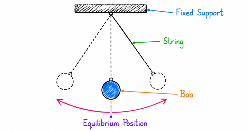
The above diagram shows a fixed support, string, central blue bob, dashed left and right swing positions, a vertical equilibrium line, and a curved arrow indicating back-and-forth motion.

Damping

Damping is the gradual loss of mechanical energy due to forces such as air resistance and friction at the pivot.

As damping removes energy, the pendulum’s maximum angle gradually becomes smaller.

---

How to Use the Simple Pendulum Simulator

The simulator provides several adjustable controls. Change one variable at a time so that you can clearly identify its effect.

1. Adjust the String Length

Use the length control to make the pendulum string shorter or longer.

Observe the animation and compare how quickly the pendulum completes each swing.

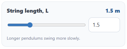
You should notice that:

• A shorter pendulum swings more quickly.
• A longer pendulum swings more slowly.
• Increasing the length increases the period.

This happens because the bob of a longer pendulum must travel along a larger path, and its motion responds differently to gravity.

---

2. Change the Bob Mass

Adjust the mass of the pendulum bob and observe the period, speed, and energy readings.

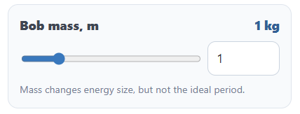
In an ideal simple pendulum:

• A heavier bob does not necessarily swing faster.
• A lighter bob does not necessarily swing more slowly.
• The period remains almost unchanged when only the mass is changed.
• The pendulum’s kinetic and potential energy values increase when its mass increases.

This is an important discovery: mass affects the amount of energy in the system, but it does not appear in the ideal small-angle period formula.

The simulator is designed to help learners observe this distinction directly.

---

3. Set the Starting Angle

The starting angle determines how far the pendulum is pulled away from its equilibrium position before being released.

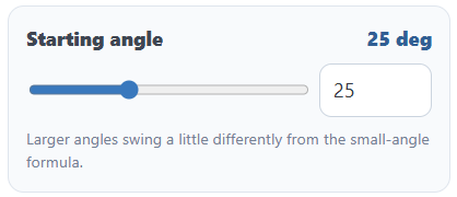
Try several starting angles and observe:

• The distance traveled by the bob
• The maximum height reached
• The pendulum’s maximum speed
• The shape of the angle-versus-time graph
• The potential and kinetic energy values

A larger angle gives the pendulum more initial gravitational potential energy because the bob begins at a greater height.

For relatively small angles, the standard pendulum-period formula provides a good approximation. At larger angles, the motion becomes less accurately described by the small-angle approximation.

---

4. Change the Strength of Gravity

Gravity supplies the restoring force that pulls the pendulum toward its equilibrium position.

Use the gravity control or available gravity presets to compare the pendulum’s motion under different gravitational conditions.

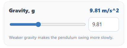
For example, compare Earth-like gravity with Moon-like gravity.

You should observe that:

• Stronger gravity produces faster oscillations.
• Weaker gravity produces slower oscillations.
• The period increases when gravitational acceleration decreases.
• The pendulum would not oscillate normally without a gravitational restoring force.

The simulator includes the option to explore how reduced gravity changes pendulum motion.

---

5. Add Damping

Increase the damping setting to represent stronger air resistance or friction.

With little or no damping, the pendulum continues swinging for a long time, and its total mechanical energy remains approximately constant.

With greater damping:

• The swing amplitude gradually decreases.
• The pendulum loses mechanical energy.
• The angle graph becomes smaller over time.
• The kinetic and potential energy values decrease.
• The pendulum eventually approaches its equilibrium position.

Damping does not mean that energy disappears. Instead, mechanical energy is transferred into other forms, mainly thermal energy in the pendulum and its surroundings.

---

6. Pause, Reset, and Compare

Use the simulator’s playback controls to pause the animation or restart an investigation.

Resetting the simulator is helpful when comparing two situations. For example:

1. Set the pendulum length to a particular value.
2. Observe or record the period.
3. Reset the simulation.
4. Change only the length.
5. Compare the new result.

Keeping all other variables constant makes the investigation a fair test.

---

The Simple Pendulum Period Formula

For relatively small swing angles, the period of a simple pendulum can be estimated using:

T ≈ 2π√(L/g)

Where:

• T is the period in seconds.
• L is the pendulum length in metres.
• g is gravitational acceleration in metres per second squared.
• π is approximately 3.1416.

The formula shows that the ideal pendulum period mainly depends on:

1. The length of the pendulum
2. The gravitational field strength

Notice that the bob’s mass is not included in the formula.

---

How Does Length Affect the Period?

The length appears inside a square root:

T ∝ √L

This means that the period does not increase in direct proportion to length.

For example, doubling the length does not double the period. Instead:

New period factor = √2 ≈ 1.41

The new period should therefore be about 1.41 times the original period.

To double the period, the pendulum length would need to be multiplied by four:

√4 = 2

You can test these relationships using the simulator.

---

How Does Gravity Affect the Period?

Gravity appears in the denominator of the period formula:

T ∝ 1/√g

This means that increasing gravity decreases the period, while decreasing gravity increases the period.

A pendulum on the Moon swings more slowly than the same pendulum on Earth because the Moon’s gravitational field is weaker.

Why Does Mass Not Affect the Ideal Period?

A heavier bob experiences a greater gravitational force than a lighter bob. However, it also has greater inertia, meaning it resists changes in motion more strongly.

In the ideal pendulum model, these effects balance in such a way that the bob’s mass cancels from the equation of motion.

As a result, pendulums of equal length released from the same small angle have approximately the same period, even when their bob masses are different.

In real experiments, small differences may still appear because of air resistance, string properties, bob size, pivot friction, or measurement error.

Energy Changes in a Pendulum

A pendulum continually transforms energy between gravitational potential energy and kinetic energy.

Gravitational Potential Energy

Gravitational potential energy depends on the bob’s height above its lowest position.

It can be represented by:

PE = mgh

Where:

• m is mass
• g is gravitational acceleration
• h is height above the reference position

Potential energy is greatest at the two highest points of the swing.

At those points:

• The bob briefly stops changing direction.
• Its speed is approximately zero.
• Its kinetic energy is at its minimum.

---

Kinetic Energy

Kinetic energy is the energy associated with motion.

It can be represented by:

KE = ½mv²

Where:

• m is mass
• v is speed

Kinetic energy is greatest at the bottom of the swing because this is where the bob moves fastest.

At the equilibrium position:

• Height is at its minimum.
• Gravitational potential energy is at its minimum.
• Speed is at its maximum.
• Kinetic energy is at its maximum.

---

Total Mechanical Energy

Total mechanical energy is the sum of kinetic and gravitational potential energy:

Total mechanical energy = KE + PE

Without damping:

• Potential energy changes into kinetic energy.
• Kinetic energy changes back into potential energy.
• Total mechanical energy remains approximately constant.

With damping, some mechanical energy is transferred to the surroundings during every swing. The simulator’s energy display helps learners observe these transformations.

---

Understanding the Angle-Versus-Time Graph

The simulator includes an angle-versus-time graph that shows how the angular position of the pendulum changes.

Horizontal axis

The horizontal axis represents time.

Moving from left to right shows how the motion develops as time passes.

Vertical axis

The vertical axis represents the pendulum’s angular displacement from equilibrium.

Positive and negative values represent opposite sides of the equilibrium position.

Peaks and troughs

A peak represents the maximum angle on one side.

A trough represents the maximum angle on the opposite side.

The time between two consecutive peaks represents one complete period.

Zero crossings

Whenever the graph crosses zero, the pendulum is passing through its equilibrium position.

At these moments, the bob normally has its greatest speed.

Graph with no damping

With little or no damping, the graph maintains approximately the same height. This indicates that the amplitude remains nearly constant.

Graph with damping

When damping is added, the peaks and troughs gradually move closer to zero. This shrinking graph shows that the oscillation amplitude and mechanical energy are decreasing.

---

Suggested Pendulum Investigations

Investigation 1: Does Mass Affect the Period?

1. Select a fixed string length.
2. Choose a small starting angle.
3. Set damping to zero or its lowest value.
4. Run the simulation with a light bob.
5. Record the period.
6. Increase the bob mass without changing anything else.
7. Compare the periods.

Question: Does increasing mass significantly change the period?

Expected observation: The energy values change, but the ideal period remains nearly the same.

---

Investigation 2: How Does Length Affect the Period?

1. Select a short string length.
2. Record the period.
3. Double the string length.
4. Record the new period.
5. Compare the two values.

Question: Does doubling the length double the period?

Expected observation: The period increases, but it does not double. It should increase by approximately a factor of √2 under ideal small-angle conditions.

---

Investigation 3: Earth Versus Moon Gravity

1. Keep the length, mass, angle, and damping constant.
2. Run the pendulum using Earth-like gravity.
3. Record the period.
4. Change to Moon-like gravity.
5. Observe the new motion and period.

Question: Why does the pendulum swing more slowly under weaker gravity?

---

Investigation 4: Mechanical Energy Conservation

1. Set damping to zero.
2. Release the pendulum from a moderate angle.
3. Observe the kinetic and potential energy displays.
4. Watch the total mechanical energy.

Questions:

• Where is potential energy greatest?
• Where is kinetic energy greatest?
• Does the total mechanical energy remain approximately constant?

---

Investigation 5: The Effect of Damping

1. Begin with no damping.
2. Observe the amplitude and energy graph.
3. Add a small amount of damping.
4. Repeat with stronger damping.
5. Compare how quickly the pendulum slows down.

Question: How does increasing damping affect the amplitude, energy, and time taken for the pendulum to settle?

---

Investigation 6: Starting Angle and Motion

1. Choose a small starting angle.
2. Record the period.
3. Increase the starting angle substantially.
4. Compare the period and graph.

Question: At what point do you begin to notice that the period is no longer almost independent of the starting angle?

This investigation introduces learners to the limits of the small-angle approximation.

---

Real-World Applications of Pendulums

Pendulum motion has been used in many scientific and engineering applications.

Pendulum clocks

Traditional pendulum clocks use the regular timing of a pendulum to regulate their mechanisms.

Metronomes

Mechanical metronomes use oscillatory motion to produce regular beats for musicians.

Seismometers

Some instruments used to detect ground movement rely on inertia and pendulum-like suspended masses.

Playground swings

A playground swing behaves similarly to a pendulum, although the rider’s body movements and the flexible supports make it more complicated than an ideal pendulum.

Foucault pendulum

A Foucault pendulum demonstrates Earth’s rotation. As the pendulum continues swinging, its plane of oscillation appears to rotate relative to the ground.

Engineering vibration studies

Pendulum-like systems help engineers study oscillations, damping, resonance, stability, and vibration control.

---

Learning Outcomes

After using the Simple Pendulum Simulator, learners should be able to:

• Define period, frequency, amplitude, equilibrium, oscillation, and damping.
• Explain why longer pendulums swing more slowly.
• Describe how gravity affects pendulum timing.
• Recognize that bob mass changes energy but not the ideal period.
• Identify where kinetic and potential energy are greatest.
• Explain the conservation of mechanical energy in an undamped system.
• Interpret an angle-versus-time graph.
• Describe how damping reduces amplitude and mechanical energy.
• Conduct a fair test by changing one variable at a time.
• Recognize the limitations of the small-angle pendulum formula.

---

Conclusion

The Simple Pendulum Simulator turns an important physics model into an interactive experiment. By adjusting string length, bob mass, starting angle, gravity, and damping, learners can immediately observe how different variables influence oscillatory motion.

The central lesson is that the period of an ideal pendulum mainly depends on its length and the gravitational field strength—not on the bob’s mass. At the same time, the simulator shows how energy continuously changes between gravitational potential energy and kinetic energy during every swing.

Experiment with one setting at a time, study the animation and graph, and use the investigation questions to discover the physics behind pendulum motion.